
Axis-Aligned Bounding Boxes for Continuous Distributions
The Algorithm
I'll describe the algorithm and demonstrate its use through the following example problem.Consider a set of $N$ two dimensional spherical Normal distributions with center $\mu_i$ and variance $\sigma_i$, $\mathcal{N}(\mu_i, \sigma_i)$. Say we are interested in computing the following matrix, which has entries corresponding to the following integral for all $N^2$ pairs of distributions (abbreviated $\mathcal{N}_i$ for simplicity): $$S_{ij} = \int_{\Omega} \mathcal{N}_i \mathcal{N}_j d\mathbf{r},$$ where $\Omega$ denotes the entire quadrature grid and $d\mathbf{r}$ indicates integration over all dimensions of $\mathcal{N}_i$.
Due to the Gaussian nature of these distributions, $S_{ij}$ can be computed analytically. But, let's suppose that we have to compute $S_{ij}$ via numerical quadrature, i.e. on a grid. In many physical applications, these distributions typically cannot be too close to eachother, or $\mu_i - \mu_j > d$ for some distance $d$. Forming $S$ would then require $N^3$ compute time; for each of the $N^2$ matrix entries we would compute an integral on a grid that scales with $N$.
However, for large sets of distributions where $\sigma_i$ is small compared to the average distance between distribution centers, each distribution is nearly zero on the vast majority of the quadrature grid. We introduce the parameter $\epsilon$ and define the compact support of $\mathcal{N}_i$ as the "smallest" $\Omega_i$ such that the following inequality is satisfied, $$\int_{\Omega_i} \mathcal{N}_i d\mathbf{r} > 1 - \epsilon,$$ where the integration is done over $\Omega_i$ rather the entire quadrature grid $\Omega$.
$\epsilon = 0$ implies that $\Omega_i$ is the entire quadrature grid because $\int \mathcal{N}_i d\mathbf{r} = 1$. On the other hand, $\epsilon > 0$ yields $\Omega_i$ that can be significantly smaller than $\Omega$. A small nonzero $\epsilon$ implies that $\mathcal{N}_i$ outside of $\Omega_i$ is negligable. Turning back to our original problem, $S_{ij}$ need only be computed on a domain where both $\mathcal{N}_i$ and $\mathcal{N}_j$ are non-negligable. This implies that $S_{ij}$ can be computed on the the intersection of $\Omega_i$ and $\Omega_j$, $\Omega_{ij} = \Omega_i \cap \Omega_j$. There are other choices here, but this is perhaps the simplest.
This definition has two important consequences. Firstly, $S_{ij}$ is only non-zero when $\Omega_{ij}$ itself is non-zero. Secondly, computation of $S_{ij}$ using $\Omega_{ij}$ is now independent of the total number of distributions $N$. As such, given the list of all $\Omega_i$ and all interacting pairs, computing the matrix $S$ scales linearly with $N$. Computing all $\Omega_i$ and all interaction pairs can be done in $\mathcal{O}(N)$ time as well with more work, but this is typically unnecessary.
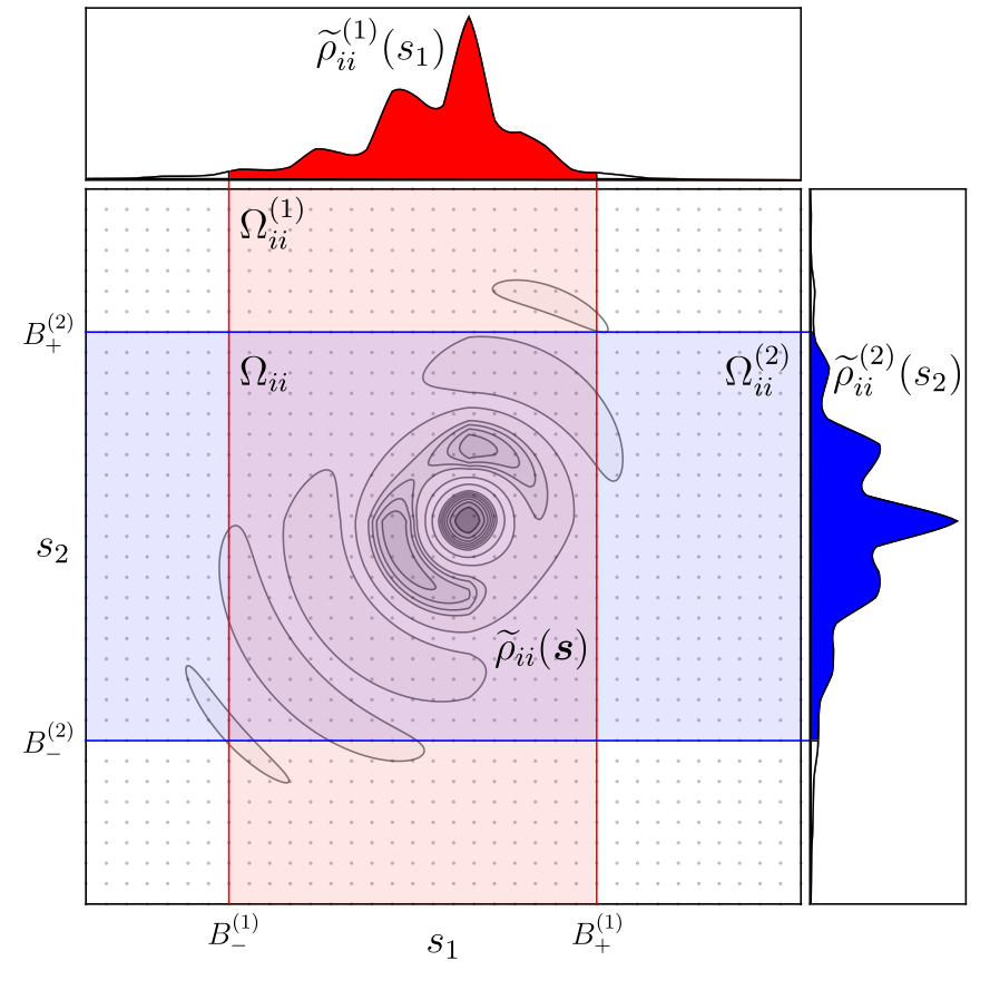
But how is $\Omega_i$ actually computed? It's practical to constrain $\Omega_i$ to be a box aligned with the axes of the quadrature grid. This allows us to transform the problem of finding $\Omega_i$ into several subproblems, one for each dimension of the distribution. The steps are as follows: 1) For each dimension of the distribution, construct a marginal distribution that integrates over all other coordinates. For example, the first marginal distribution for a 2D Normal distribution would be $$ \mathcal{N}_x = \int \mathcal{N}_i dy $$ 2) For each marginal distribution, find the marginal bounding box. This is done by incrementally adding points of the marginal distribution, starting with the grid point with the highest marginal distribution value. Then, add the next largest. Continue adding until the sum (Reiman integral) reachest a value greater than $1-\epsilon/n$, where $n$ is the distribution dimension. The marginal bounding box is the smallest continuous set that contains all of the added points. 3) The final axis-aligned bounding box is the intersection of all of the marginal bounding boxes.
In practice, the marginal bounding box algorithm looks like the function below, which returns a list containing the left and rightmost bounds of the marginal bounding box.
def marginal_bound(dist, eps):
    dist_norm = np.sum(dist)
    pos_list = list(range(len(dist)))
    center = sum([d*pos for d, pos in zip(dist, pos_list)])
    cost_list = [len(dist) - np.abs(c - center) for c in pos_list]
    dist_to_sort = np.array(list(zip(dist, cost_list)))
    ordering = np.argsort(dist_to_sort, order=['dist','cost'], stable=True)[::-1]

    norm = 0
    lb = max(ordering)
    rb = min(ordering)
    i = 0
    while norm < (1.0 - eps)*dist_norm:
        norm += dist[ordering[i]]
        lb = min(ordering[i], lb)
        rb = max(ordering[i], rb)
        i += 1
    return [lb.item(),(rb + 1).item()]
This algorithm works on any dimensional distribution, even those that don't decay monotonically. As seen in the figure below, the two marginal bounding boxes (red and blue regions) combine to form the final axis-aligned bounding box (intersection of red and blue, purple region).
A Concrete Example
We can make this more concrete with an example. Consider the set of $100$ $\mathcal{N}_i$ shown below, all with $\sigma_i=0.5$. We use $\epsilon=0.01$ here, but this parameter can be adjusted depending on the desired accuracy.
import aabb
import numpy as np
import math
from scipy.stats import multivariate_normal
import random
import matplotlib.pyplot as plt

random.seed(42)

# Generate distributions
distribution_grid_size = 10
distributions = []
coords = []
for x in range(distribution_grid_size):
    for y in range(distribution_grid_size):
        x_rand, y_rand = [random.random(), random.random()]
        coords.append([x + x_rand, y + y_rand])
        dist = multivariate_normal([x + x_rand, y + y_rand],[[0.5,0.0],[0.0,0.5]])
        distributions.append(dist)

n_distributions = len(distributions)

# Generate grid
quadrature_spacing = 0.1
quadrature_padding = 4
minpos = 0 - quadrature_padding
maxpos = distribution_grid_size + quadrature_padding
x1, x2 = np.mgrid[minpos:maxpos:quadrature_spacing, minpos:maxpos:quadrature_spacing]
volume_element = quadrature_spacing**2
pos = np.stack((x1, x2), axis=2)
Here is a visualization of those distributions, where the black dots denote the center of the distribution, and the gray circles indicate the spread.

# Compute AABBs
epsilon = 0.01
aabbs = []
for d in distributions:
    d_on_grid = np.array(volume_element*d.pdf(pos))
    d_aabb = aabb.draw_aabb(d_on_grid, epsilon)
    aabbs.append(d_aabb)
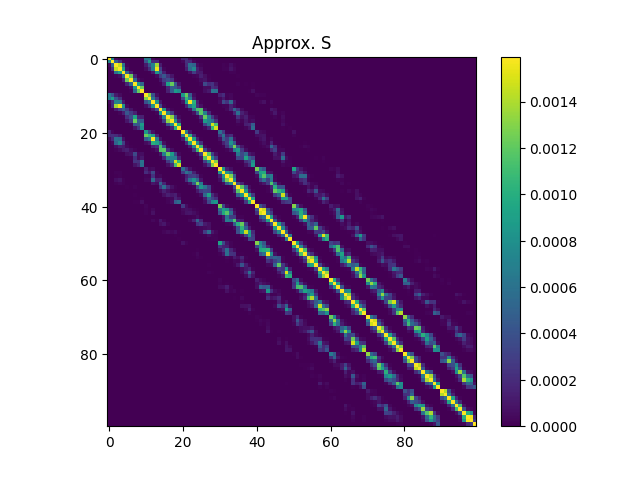
Given this list, we can loop through all $\mathcal{N}_i$ pairs and compute the finite $\Omega_{ij}$ and $S_{ij}$.
s_approx = np.full((n_distributions, n_distributions), 0.0)
for i,bi in enumerate(aabbs):
    for j,bj in enumerate(aabbs):
        if i >= j:
            int_bounds = aabb.aabb_intersection(bi, bj)
            if int_bounds != None:
                trunc_i = aabb.trunc_dist(np.array(volume_element*distributions[i].pdf(pos)), int_bounds)
                trunc_j = aabb.trunc_dist(np.array(volume_element*distributions[j].pdf(pos)), int_bounds)
                s_approx[i,j] = np.sum(trunc_i * trunc_j)
                s_approx[j,i] = s_approx[i,j]
This results in the following $S$ matrix.
Check out the GitHub Repo!